Fun Math

Gauss Quadrature

The following is a simplied case of the fundamental theorem from wikipedia, and its proof.

If \(p_n\) is a polynomial of degree \(n\) such that \begin{eqnarray} \int_{-1}^1 x^k p_n(x)\,dx=0\qquad \forall k=0, 1, 2, \ldots, n-1, \end{eqnarray} and \(\{x_i\}\) are roots of \(p_n\), then there is a set of weights \(\{w_i\}\) such that

\[\int_{-1}^1 h(x)\,dx = \sum_{i=1}^n h(x_i)w_i\]

for all polynomial \(h\) of degree \(2n-1\).

To prove, first write

\[\underbrace{h(x)}_{\text{of degree } 2n-1} = \underbrace{p_n(x)}_{n}\underbrace{q(x)}_{n-1}+\underbrace{r(x)}_{n-1}.\]

Thus

\[\int_{-1}^1 h(x)\,dx = \underbrace{\int_{-1}^1 p_n(x)q(x)\,dx}_{= 0} + \int_{-1}^1 r(x)\,dx.\]

The first term of the right hand side vanishes. On the other hand, we also have

\[\sum_{i=1}^n h(x_i)w_i = \underbrace{\sum_{i=1}^n p_n(x_i)q(x_i)w_i}_{=0} + \sum_{i=1}^n r(x_i)w_i\]

since \(\{x_i\}\) are roots of \(p_n(x)\). It remains to prove there is a set of weights \(\{w_i\}\) such that

\[\int_{-1}^1 r(x)\,dx = \sum_{i=1}^n r(x_i)w_i\]

for all polynomial \(r(x)\) of degree \(n-1\), which is true if and only if

\[\int_{-1}^1 x^k\,dx = \sum_{i=1}^n x_i^k w_i\qquad\forall k=0, 1, 2, \ldots, n-1.\]

Set \(I_k = \int_{-1}^1 x^k\,dx\). The above can be written as a linear system

\[\begin{split}\begin{pmatrix} 1 & 1 & 1 & \cdots & 1 \\ x_1 & x_2 & x_3 & \cdots & x_n \\ x_1^2 & x_2^2 & x_3^2 & \cdots & x_n^2 \\ \vdots & \vdots & \vdots & \ddots & \vdots \\ x_1^{n-1} & x_2^{n-1} & x_3^{n-1} & \cdots & x_n^{n-1} \end{pmatrix} \begin{pmatrix} w_1\\ w_2\\ w_3\\ \vdots\\ w_n \end{pmatrix} = \begin{pmatrix} I_0\\ I_1\\ I_2\\ \vdots\\ I_{n-1} \end{pmatrix}.\end{split}\]

The existence of \(\{w_i\}\) is obvious since the matrix is invertible.

An Interesting Property of 13

If you reverse its digits and then find square, or if you reverse the digits of its square, the results are the same: \begin{align*} 13^2 &= 169, \\ 31^2 &= 961. \end{align*} Other examples of numbers with this property are 12 and below:

n = 20101001

int(str(n**2)[::-1]) == int(str(n)[::-1])**2

True

The following two examples are a bit surprising:

n = 20211001

int(str(n**2)[::-1]) == int(str(n)[::-1])**2

True

n = 20211002

int(str(n**2)[::-1]) == int(str(n)[::-1])**2

False

A Somewhat Counterintuitive Result

Let \(X_t\) be the solution of \(dX_t = X_t dW_t\) with \(X_0 = 1\). Then \begin{align*} X_t = e^{-\frac{t}{2} + W_t} \rightarrow 0 \qquad\text{ as }t\rightarrow \infty, \end{align*} but \(X_t\) is a martingale so \(E[X_t] = X_0 = 1\) for all \(t>0\).

Although this might seen counterintuitive at first glance, if one think about a large but finite value of \(t\), this is less so.

Closed Form Expression of the Fibonacci Numbers

令 \(\lambda_1, \lambda_2\) 為二次方程式 \(a x^2 + b x + c = 0\) 的兩根，則 \begin{align*} a \lambda_1^2 + b \lambda_1 + c = 0. \end{align*} 等號兩邊同乘 \(\lambda_1^n\) 可以得到 \begin{align*} a \lambda_1^{n+2} + b \lambda_1^{n+1} + c \lambda_1^n = 0. \end{align*} 同樣的，對 \(\lambda_2\) 也可以得到 \begin{align*} a \lambda_2^{n+2} + b \lambda_2^{n+1} + c \lambda_2^n = 0. \end{align*} 現在把上面兩個式子作線性組合： \begin{align*} 0 &= c_1(a \lambda_1^{n+2} + b \lambda_1^{n+1} + c \lambda_1^n) + c_2(a \lambda_2^{n+2} + b \lambda_2^{n+1} + c \lambda_2^n)\\ &= a \left(c_1\lambda_1^{n+2}+c_2\lambda_2^{n+2}\right) + b \left(c_1\lambda_1^{n+1}+c_2\lambda_2^{n+1}\right) + c \left(c_1\lambda_1^{n}+c_2\lambda_2^{n}\right). \end{align*} 於是可以得到以下結論：數列 \(F_n = c_1\lambda_1^{n}+c_2\lambda_2^{n}\) 滿足遞迴式 \begin{align*} \begin{cases} a F_{n+2} + b F_{n+1} + c F_{n} = 0\\ F_0 = c_1 + c_2\\ F_1 = c_1\lambda_1 + c_2\lambda_2 \end{cases} \end{align*} 其中 \(\lambda_1, \lambda_2\) 為 \(a x^2 + b x + c = 0\) 的兩根。\(a x^2 + b x + c = 0\) 就是這個遞迴式的特徵方程。 現在代入費式數列的遞迴定義 \(a=1, b=c=-1\) 可以求得 \begin{align*} \lambda_j = \frac{1\pm \sqrt{5}}{2}, \qquad j=1, 2, \end{align*} 再把 \(\lambda_1, \lambda_2\) 代入 \begin{align*} \begin{cases} F_0 = c_1 + c_2 = 0\\ F_1 = c_1\lambda_1 + c_2\lambda_2 = 1 \end{cases} \end{align*} 可以求得 \(c_1 = 1/\sqrt{5}, c_2 = -1/\sqrt{5}\)，所以 \begin{align*} F_n = \frac{1}{\sqrt{5}}\left(\left(\frac{1+\sqrt{5}}{2}\right)^n - \left(\frac{1-\sqrt{5}}{2}\right)^n\right). \end{align*}

The Solution Formula to the Riccati Equation

Assuming \(pq\neq 0\) and \(p\neq q\), the Riccati equation \begin{align*} \begin{cases} y'(t) = a(y(t) - p)(y(t) - q)\\ y(0) = 0 \end{cases} \end{align*} has a closed form “solution” \begin{align*} y(t) = pq\left(\frac{1-e^{-a(p-q)t}}{p-qe^{-a(p-q)t}}\right) \end{align*} that people use all the time, although it does not always hold. Define \begin{align*} t^* = -\frac{1}{a}\left(\frac{\log p-\log q}{p-q}\right). \end{align*} If \(t^*\) is real positive, the closed form formula is only the solution to the Riccati equation for \(t\in[0, t^*)\). This is because when \(t\) approaches \(t^*\), the denominator in the closed form formula goes to 0, making the solution infinity. Here is a numerical example: When \(a=-1, p=2, q=1\), below is a plot of the closed form formula:

import numpy as np
from pandas import DataFrame

a = -1
p = 2
q = 1

t = np.arange(0, 1, 0.01)
y = p*q*((1-np.exp(-a*(p-q)*t))/(p-q*np.exp(-a*(p-q)*t)))

ax = DataFrame({'t': t, 'y': y}).set_index('t').plot(legend=None)
ax.set(ylim=(-20, 20), xlim=(0, 0.99), xlabel='$t$', ylabel='$y(t)$')
ax.axhline(0, color='k', lw=1)
pass

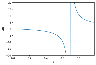
In this example we have \(t^* = \log 2 \approx 0.693147\). One can see from the plot that only before this critical time the closed form formula is the solution to the initial value problem.

If \(t^*\) is complex or if it is real negative then the closed form formula gives the solution for all \(t\ge 0\). When \(p\) and \(q\) are both real, the critical value \(t^*\) is real positive if and only if \(a\) is real negative, which is not the case in the CIR interest rate model. That is why the CIR model never runs into this issue. The Heston model with complex \(p\) and \(q\), however, is not so lucky.

Newton’s Method for Square Root Has Quadratic Convergence

For square root a simple completing the square will do the trick: \begin{align*} \frac{x + \frac{a}{x}}{2} - \sqrt{a} &= \frac12\left(x -2\sqrt{a} + \frac{a}{x}\right)\\ &= \frac12\left(\sqrt{x} - \sqrt{\frac{a}{x}}\right)^2\\ &= \frac{1}{2x}\left(x - \sqrt{a}\right)^2, \end{align*} which says the error in the next iteration is the error in this iteration squared divided by \(2x\).

A more general proof for general functions can be found on wikipedia.

Checking if an Integer Is a Perfect Square

The goal here is to prove that Newton’s method with integer division (integer division) can be used to determine if an integer is a perfect square.

This method is discussed (without proof) in a stackoverflow post, which gives the following procedure. It works for any large integer, for example 123456789**100 which is too large to convert to float for implementations relying on math.sqrt.

%%time

def is_square(a):
    x = a//2
    seen = set([x])
    while x*x != a:
        x = (x + a//x)//2
        if x in seen:
            return False
        seen.add(x)
    return True

print(is_square(123456789**100))

True
CPU times: user 12 ms, sys: 8 ms, total: 20 ms
Wall time: 16.5 ms

Assume that \(x\in\mathbb N, \sqrt{a}\in\mathbb N\) and \(x>\sqrt{a}\). With integer division, the error after one iteration is really \begin{align*} \frac{x+\frac{a - r_1}{x} - r_2}{2} - \sqrt{a} &= \frac{x+\frac{a}{x}}{2} - \sqrt{a} -\left( \frac{r_1}{2x} + \frac{r_2}{2}\right)\\ &= \frac{1}{2x}\left(x - \sqrt{a}\right)^2 - \left( \frac{r_1}{2x} + \frac{r_2}{2}\right), \end{align*} where \(r_1\) and \(r_2\) are the remainders from the division. Since they must satisfy \(r_1 < x\), \(r_2\leq 1\), we have \(r_1/(2x) + r_2/2 < 1/2 + 1/2 = 1\). Now note that this error is an integer, so we can write \begin{align*} \frac{x+\frac{a - r_1}{x} - r_2}{2} - \sqrt{a} &= \left \lfloor\frac{1}{2x}\left(x - \sqrt{a}\right)^2 \right \rfloor. \end{align*}

Simulation

This is to confirm the following is correct: \begin{align*} \text{cov}\left(\int_0^T t\,dW_t, \int_0^T W_t \,dt\right) = \frac{T^3}{6}, \end{align*} which is 1.3333 if \(T=2\) like in the below simulation.

Recall that \(E(W(t)W(s)) = s\land t\). Roughly speaking, \begin{align*} E\left(\int_0^T t\,dW_t\int_0^T W_t dt\right) &= E\left(\int_0^T\int_0^T s W_t \,dW_sdt\right)\\ &\approx E\left(\sum_i\sum_j s_j W(t_i) (W(s_{j+1}) - W(s_j)) \Delta t\right)\\ &\approx \sum_i\sum_j s_j \left[E(W(t_i)W(s_{j+1})) - E(W(t_i)W(s_j))\right] \Delta t \\ &\approx \sum_i\sum_j s_j \left[ \Delta s1_{\{t_i>s_j\}} \right] \Delta t \\ &\approx \iint\limits_{t>s} s \,ds dt = \frac{T^3}{6}. \end{align*}

%%time
import numpy as np
from scipy.stats import norm
from pandas import Series

n = 10000
T = 2

sample_size = 10000
sample = []
for i in range(sample_size):
    w = Series(norm.rvs(loc=0, scale=np.sqrt(T/n), size=n).cumsum()).shift(1, fill_value=0)
    w.index = w.index*T/n
    t = w.index
    sample.append((w.diff().dropna().values @ t[1:].values, w.sum()*T/n))

print(np.cov(np.array(sample).T))

[[2.65784801 1.33743398]
 [1.33743398 2.68333453]]
CPU times: user 23.2 s, sys: 41.1 ms, total: 23.2 s
Wall time: 24 s

Inverse Mills Ratio

We have the conditional expectation \begin{align*} E[X|X>K] &= \frac{f_X(K)}{1-F_X(K)}, \\ E[X|X where the last one is what’s known as the inverse Mills ratio taking negative. Below is a simulation using the standard normal distribution.

from numpy.random import normal
from scipy.stats import norm
n = 1000000
K = 1.5

a = norm.rvs(loc=0, scale=1, size=n)

print(a[a < K].mean())
print(-norm.pdf(K)/(norm.cdf(K)))

-0.13895207849237406
-0.13878975045885078

Calculate the 41st Root in 1 Second

Python integer can be arbitrarily large. Below is \(54^{41}\).

54**41

106695020879414327538426959056889063841348427743537143096812648481685504

Generate a random integer between \([0, 100)\) and compute its 41st power.

import random

a = random.randrange(100)
a**41

3574546132030870770399332670577487090810665965922351838949846024192

The answer is

a

44

\(3^4\) vs. \(4^3\) which one is bigger?

（和常見的微分作法不同）

\begin{eqnarray*} \frac{d}{da} a^b &=& a^b\left(\frac{b}{a}\right)\\ \frac{d}{db} a^b &=& a^b\ln a \end{eqnarray*} so \begin{eqnarray*} (a+h)^b &\approx& a^b + h(a^b\left(\frac{b}{a}\right))\\ a^{b+h} &\approx& a^b + h(a^b\ln a) \end{eqnarray*}

從 \(3^3\) 開始，要把 1 加在底數還是指數會讓值變得更大？（相當於 \(a=b=3, h=1\)）看上面的式子可以猜到加在指數更好，也就是 \(3^4\) 較大。

泰展多寫幾項也可以比出 \(e^{\pi} > \pi^e\)。和微分作法一樣可以推出更一般的結論：當指數和底數都大於 \(e\) 時，指數比較大者數值就比較大。但像 \(2.5^3\) 和 \(3^{2.5}\) 這種兩個數分別在 \(e\) 的左右時微分作法比不出來，這裡的泰展作法比較好比。不過泰展本來就是在計算數值，有點作弊。

Square Root of a Complex Number

If \(x\ge 0\), \(y\ge 0\) then \begin{align*} \sqrt{x+yi} = \sqrt{\frac{\sqrt{x^2+y^2}+x}{2}} + i \sqrt{\frac{\sqrt{x^2+y^2}-x}{2}}. \end{align*} This can be used to find the numerical values like \(\sqrt{2+17i} = 3.0917 + 2.74929i\).

\(\cos(1^\circ)\) in Closed Form

用三倍角公式和 \(\cos(60^\circ)=1/2\) 加上卡當諾公式可以算出 \(\cos(20^\circ)\) 的 closed form。再利用 \(\sin(18^\circ)=(-1+\sqrt 5)/4\) 跟和角公式可以算出 \(\cos(2^\circ) = \cos(20^\circ - 18^\circ)\)。最後用半角公式，可以算出

:nbsphinx-math:`begin{align*} cos(1^circ) = sqrt{frac{1}{2} left(1+frac{1}{4} sqrt{frac{1}{2} left(5+sqrt{5}right)}

left(sqrt[3]{frac{1}{2} left(1-i sqrt{3}right)}+sqrt[3]{frac{1}{2} left(1+i sqrt{3}right)}right)+frac{1}{4} left(sqrt{5}-1right) sqrt{1-frac{1}{4} left(sqrt[3]{frac{1}{2} left(1-i sqrt{3}right)}+sqrt[3]{frac{1}{2} left(1+i sqrt{3}right)}right)^2}right)}

end{align*}`

但是有 \(i\) 在三次根號裡開不出來，所以有這個公式還是沒辦法用古典的方法把數值算出來。\(\cos(1^\circ)\) 的數值大約是 0.999848。

為了計算 \(\cos(1^\circ)\) 的數值，與其設計複數直式開立方來計算上面這個公式的值，還不如設計直式解三次方式程求 \(\cos(20^\circ)\)。有沒有辦法直接直式計算 \(\cos(x^\circ)\)？

把 \(\cos(30^\circ)=\sqrt{3}/2\) 拿來套半角公式算出 \(\cos(15^\circ)\)，再用 \(\cos(18^\circ)\) 的值和合角公式就可以算出 \begin{align*} \cos(3^\circ) = \frac{1}{8} \left(\sqrt{2-\sqrt{3}} \left(\sqrt{5}-1\right)+\sqrt{2 \left(2+\sqrt{3}\right) \left(5+\sqrt{5}\right)}\right) \end{align*} 這個是真正的 closed form，沒有任何複數，可以直接用這個公式算出數值。有了這個值，再用卡當諾公式解 \(4x^3-3x = \cos(3^\circ)\) 就得到 :nbsphinx-math:`begin{align*} cos(1^circ) &= frac{1}{4} left(sqrt[3]{sqrt{2-sqrt{3}} left(sqrt{5}-1right)+sqrt{2 left(2+sqrt{3}right) left(5+sqrt{5}right)}-2 sqrt{-8+sqrt{3}+sqrt{15}-sqrt{frac{1}{2}

left(5+sqrt{5}right)}+sqrt{frac{1}{2} left(25+5 sqrt{5}right)}}}right.\ &+left.sqrt[3]{sqrt{2-sqrt{3}} left(sqrt{5}-1right)+sqrt{2 left(2+sqrt{3}right) left(5+sqrt{5}right)}+2 sqrt{-8+sqrt{3}+sqrt{15}-sqrt{frac{1}{2} left(5+sqrt{5}right)}+sqrt{frac{1}{2} left(25+5 sqrt{5}right)}}}right)

end{align*}` 這個公式乍看之下沒有複數但實際上是作弊的因為根號裡面有負數。結果就是這個公式的數值還是沒辦法用直式開方法算出來。